Newton–Raphson method

Here is a example about Newton-Raphson’s method in optimization. I simulated data from Poisson distribution. Under GLM framework, I compare MLE estimation by Newton-Raphson method and by statsmodels library.

Assume that \(Y\sim\text{Poisson}(10)\),

\[\begin{equation} log(E(y)) = \beta_0 \tag{1} \end{equation}\]

\[\begin{equation} E(y) = \lambda \tag{2} \end{equation}\]

From (1) and (2), \[\begin{equation} \lambda = e^{\beta_0} \tag{3} \end{equation}\]

\[\begin{equation} P(Y=y)=\frac{\lambda^{y} e^{-\lambda}}{y !} \tag{4} \end{equation}\]

Likelihood function is

\[\begin{equation} P(\mathbf{Y}=\mathbf{y})=\frac{\lambda^{\sum_{i}y_i} e^{-n\lambda}}{\prod_i y_i !} \tag{5} \end{equation}\]

Log-likelihood function is

\[\begin{equation} \ell(\lambda|\mathbf{Y}) = \sum_{i}y_i log(\lambda)-n\lambda-\sum_{i}log(y_i !) \propto \sum_{i}y_i log(\lambda) - n\lambda \tag{6} \end{equation}\]

Plot about partial log-likelihood function,\(\sum_{i}y_i log(\lambda) - n\lambda\),is shown below.

import numpy as np
import matplotlib.pyplot as plt
import numdifftools as nd
import statsmodels.api as sm
import statsmodels
np.random.seed(509)
y = np.random.poisson(lam = 10, size = 1000)
x = np.ones(1000)
def loglikelihood(x):
  l = np.exp(x)
  n = len(y)
  f1 = (np.sum(y)) * np.log(l)
  f2 = -n * l
  output = f1 + f2
  output = -output
  return output
plt.figure()
plt.plot(np.arange(2.1,2.5,0.01),
loglikelihood(np.arange(2.1,2.5,0.01)))
plt.title("Partial log-likelihood of Poisson(10)")
plt.xlabel("lambda")
plt.show()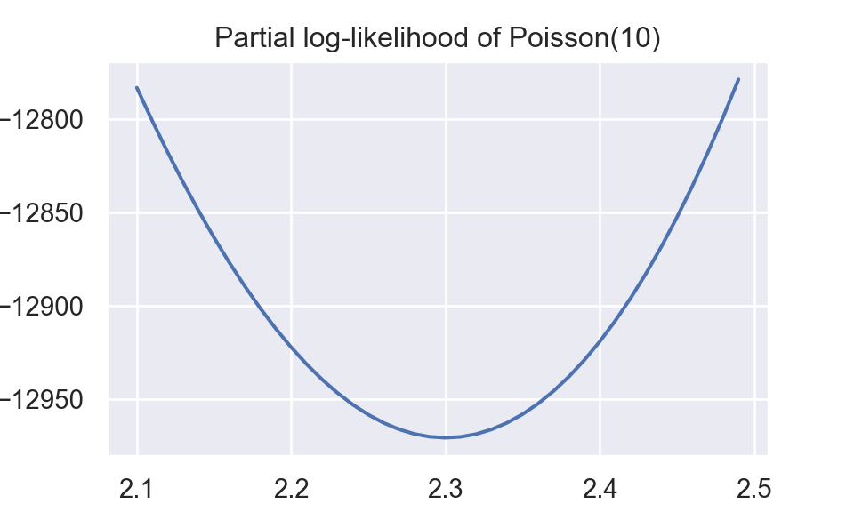

##approximation of first/second order derivative
def derivative(x):
  output = nd.Derivative(loglikelihood)
  return output(x)
def hess(x):
  output = nd.Derivative(loglikelihood, n = 2)
  return output(x)
  
##begin of newton-raphson
def newton(x0,tol=1e-10):
  diff = 100
  xold = np.copy(x0)
  xnew = 0
  i = 1
  while diff > tol:
    xnew = xold - derivative(xold)/hess(xold)
    diff = np.sum(np.abs(xnew - xold))
    xold = xnew
    print("iteration:"+str(i)+" || "+ "betas:" + str(xnew))
    print("change: {:.4f}".format(derivative(xold)/hess(xold)))
    i = i + 1
  output = {"beta":xnew, "sd":1/np.sqrt(hess(xnew))}
  return output

output = newton(2.5)

## iteration:1 || betas:2.318879946271993
## change: 0.0185
## iteration:2 || betas:2.300355926680922
## change: 0.0002
## iteration:3 || betas:2.3001822234658786
## change: 0.0000
## iteration:4 || betas:2.300182208377783
## change: 0.0000
## iteration:5 || betas:2.3001822083777355
## change: 0.0000

output

## {'beta': 2.3001822083777355, 'sd': 0.01001202164328345}

We have \(\hat{\beta}\) and var\((\hat{\beta})\), that are identical with those from statsmodels.discrete.discrete_model.Poisson.

Theoretically, \(\beta=log(\lambda)|_{\lambda=10}=2.302585\)

model = statsmodels.discrete.discrete_model.Poisson(y,x)
model.fit().summary()

Poisson Regression Results
Dep. Variable:	y	No. Observations:	1000
Model:	Poisson	Df Residuals:	999
Method:	MLE	Df Model:	0
Date:	Sat, 25 Feb 2023	Pseudo R-squ.:	0.000
Time:	22:18:43	Log-Likelihood:	-2538.4
converged:	True	LL-Null:	-2538.4
Covariance Type:	nonrobust	LLR p-value:	nan

	coef	std err	z	P>\|z\|	[0.025	0.975]
const	2.3002	0.010	229.742	0.000	2.281	2.320

Newton–Raphson method

Kevin Liu

5/09/2020