Expectation Maximization Algorithm - with one example
Kevin Liu
8/30/2018
Expectation Maximization Algorithm is a very important algorithm for mixture distribution. Here I derive the general form/step for mixture distribution with 2 distributions.
1 General form of EM algorithm for mixture distribution with 2 parts.
For \(\mathbf{x} = (x_1,\dots,x_n)\), where \(x_i\) is known, with \(f_0\) and \(f_1\) being probability density functions. We assume that \[\begin{equation} f_{X_i}(X_i = x_i) = \pi_0 f_0(x_i) + \pi_1 f_1(x_i) \tag{1.1} \end{equation}\]
Important relationship between \(\pi_0\) and \(\pi_1\) \[\begin{equation} \pi_0 + \pi_1 = 1 \tag{1.2} \end{equation}\]
Define \(\boldsymbol{\theta}\) is a vector containing all parameters of \(f_0(x_i)\) and \(f_1(x_i)\).
Define \(Z_i\) as group information, which is unknown. The complete mixture probability distribution function is
\[\begin{equation} f(x_i,Z_i;\boldsymbol{\theta}) = \mathbf{I}(Z_i = 0 | \mathbf{X}, \boldsymbol{\theta})\pi_0 f_0(x_i) + \mathbf{I}(Z_i = 1 | \mathbf{X}, \boldsymbol{\theta})\pi_1 f_1(x_i) \tag{1.3} \end{equation}\]
Complete likelihood function
\[\begin{equation} L(\boldsymbol{\theta}; \mathbf{X},\mathbf{Z}) = \prod_{i=1}^{n} [\mathbf{I}(Z_i = 0 | \mathbf{X}, \boldsymbol{\theta})\pi_0 f_0(x_i) + \mathbf{I}(Z_i = 1 | \mathbf{X}, \boldsymbol{\theta})\pi_1 f_1(x_i)] \tag{1.4} \end{equation}\]
Complete log-likelihood function \[\begin{equation} \begin{split} \ell(\boldsymbol{\theta}; \mathbf{X},\mathbf{Z}) &= \text{log}[\prod_{i=1}^{n} [\mathbf{I}(Z_i = 0 | \mathbf{X}, \boldsymbol{\theta})\pi_0 f_0(x_i) + \mathbf{I}(Z_i = 1 | \mathbf{X}, \boldsymbol{\theta})\pi_1 f_1(x_i)]] \\ &= \sum_{i=1}^{n} \text{log}[\mathbf{I}(Z_i = 0 | \mathbf{X}, \boldsymbol{\theta})\pi_0 f_0(x_i) + \mathbf{I}(Z_i = 1 | \mathbf{X}, \boldsymbol{\theta})\pi_1 f_1(x_i)] \\ &= \sum_{i=1}^{n} \mathbf{I}(Z_i = 0 | \mathbf{X}, \boldsymbol{\theta})\text{log}[\pi_0 f_0(x_i)] + \mathbf{I}(Z_i = 1 | \mathbf{X}, \boldsymbol{\theta})\text{log}[\pi_1 f_1(x_i)] \end{split} \tag{1.5} \end{equation}\]
The last step of (1.5) is true because \(Z_i\) could be either \(0\) or \(1\), but \(Z_i\) can not be \(0\) and \(1\) simultaneous.
The E step:
The E step is about calculating expected value of the log-likelihood function of \(\boldsymbol{\theta}\), with respect to the current conditional distribution of \(\mathbf{Z}\) given \(\mathbf{X}\) and the current estimates of the parameters \(\boldsymbol{\theta}^{(t)}\). The red highlighted part is extremely important.
\[\begin{equation} \begin{split} Q(\boldsymbol{\theta} | \boldsymbol{\theta}^{(t)}) & = E_{\mathbf{Z}|\mathbf{X}, \boldsymbol{\theta}^{(t)}}[\ell(\boldsymbol{\theta}^{(t)}; \mathbf{X},\mathbf{Z})] \\ &= E_{\mathbf{Z}|\mathbf{X}, \boldsymbol{\theta}^{(t)}} [\sum_{i=1}^{n} \mathbf{I}(Z_i = 0 | \mathbf{X}, \boldsymbol{\theta}^{(t)})\text{log}[\pi_0 f_0(x_i)] + \mathbf{I}(Z_i = 1 | \mathbf{X}, \boldsymbol{\theta}^{(t)})\text{log}[\pi_1 f_1(x_i)]] \\ &\stackrel{(A.1)}{=} \sum_{i=1}^{n}E_{\mathbf{Z}|\mathbf{X}, \boldsymbol{\theta}^{(t)}} [\mathbf{I}(Z_i = 0 | \mathbf{X}, \boldsymbol{\theta}^{(t)})\text{log}[\pi_0 f_0(x_i)] + \mathbf{I}(Z_i = 1 | \mathbf{X}, \boldsymbol{\theta}^{(t)})\text{log}[\pi_1 f_1(x_i)]] \\ &\stackrel{(A.2)}{=} \sum_{i=1}^{n} \text{log}[\pi_0 f_0(x_i)] E_{\mathbf{Z}|\mathbf{X}, \boldsymbol{\theta}^{(t)}}[\mathbf{I}(Z_i = 0 | \mathbf{X}, \boldsymbol{\theta}^{(t)})] + \text{log}[\pi_1 f_1(x_i)] E_{\mathbf{Z}|\mathbf{X}, \boldsymbol{\theta}^{(t)}}[\mathbf{I}(Z_i = 1 | \mathbf{X}, \boldsymbol{\theta}^{(t)})]\\ &\stackrel{(A.3)}{=} \sum_{i=1}^{n} \text{log}[\pi_0 f_0(x_i)] P(\mathbf{I}(Z_i = 0 | \mathbf{X}, \boldsymbol{\theta}^{(t)})) + \text{log}[\pi_1 f_1(x_i)] P(\mathbf{I}(Z_i = 1 | \mathbf{X}, \boldsymbol{\theta}^{(t)}))\\ &\stackrel{(A.4)}{=} \sum_{i=1}^{n} \text{log}[\pi_0 f_0(x_i)] T_{i,0} + \text{log}[\pi_1 f_1(x_i)] T_{i,1} \end{split} \tag{1.6} \end{equation}\]
The M step is relatively easy. It is about finding the parameters that maximize this quantity.
\[\begin{equation} \begin{split} \boldsymbol{\theta}^{(t+1)} = \text{argmax} Q(\boldsymbol{\theta} | \boldsymbol{\theta}^{(t)}) \end{split} \tag{1.7} \end{equation}\]
2 Example
This example comes from Prof.Zhao who works in Temple University and introduced me the EM algorithm. He made an good homework for EM. I decide to share the homework.
Assume
\[\begin{equation} \begin{cases} f_0(x_i) = 1(0 \le x_i \le 1)\\ f_1(x_i)=\beta(1-x_i)^{\beta-1} \end{cases} \tag{2.1} \end{equation}\]
(1.6) becomes
\[\begin{equation} \begin{split} Q(\boldsymbol{\theta} | \boldsymbol{\theta}^{(t)}) &= \sum_{i=1}^{n} T^{(t)}_{0,i} \text{log}(\pi_0 \times 1) + T^{(t)}_{1,i} \text{log}(\pi_1 \times \beta(1-x_i)^{\beta-1})\\ &\stackrel{(1.2)}{=} \sum_{i=1}^{n} T^{(t)}_{0,i} \text{log}(\pi_0 \times 1) + T^{(t)}_{1,i} \text{log}((1-\pi_0) \times \beta(1-x_i)^{\beta-1}) \end{split} \tag{2.2} \end{equation}\]
From calculus, we know that first derivatives must be 0. (Note: \(T^{(t)}_{j,i}\), which is defined in appendix A.4, should be treated as constant)
\[\begin{equation} \frac{\partial Q(\boldsymbol{\theta} | \boldsymbol{\theta}^{(t)})}{\partial \pi_0} = \sum_{i=1}^{n} T^{(t)}_{0,i} \frac{1}{\pi_0} + \sum_{i=1}^{n} T^{(t)}_{1,i} \frac{1}{\pi_0 - 1} = 0 \tag{2.3} \end{equation}\]
This implies
\[\begin{equation} \pi_0^{(t+1)} = \frac{\sum_{i=1}^{n} T^{(t)}_{0,i}}{\sum_{i=1}^{n} T^{(t)}_{0,i} + \sum_{i=1}^{n} T^{(t)}_{1,i}} = \frac{\sum_{i=1}^{n} T^{(t)}_{0,i}}{\sum_{i=1}^{n} ( T^{(t)}_{0,i} + T^{(t)}_{1,i})} = \frac{\sum_{i=1}^{n} T^{(t)}_{0,i}}{n} \tag{2.4} \end{equation}\]
Similarly, we have that
\[\begin{equation} \frac{\partial Q(\boldsymbol{\theta} | \boldsymbol{\theta}^{(t)})}{\partial \beta} = \sum_{i=1}^{n} T^{(t)}_{1,i} (\frac{1}{\beta} + log(1-x_i)) = 0 \tag{2.5} \end{equation}\]
This implies
\[\begin{equation} \beta^{(t+1)} = \frac{\sum_{i=1}^{n} T^{(t)}_{1,i}}{-\sum_{i=1}^{n} T^{(t)}_{1,i} log(1-x_i)} \tag{2.6} \end{equation}\]
2.1 Example - Calculation by R
Create a loop in R to get \(\pi_0\) and \(\beta\).
With initial value of \(0.69\) and \(11\), at 32th iteration, \(\pi_0 = 0.69679\) and \(\beta = 11.09328\). (Initial value are chosen on purpose so it doesn’t require too many iterations until converge).
Link:pvalue.csv. Note that pvalue.csv is simulated data.
pvalue <- read.csv("files/pvalue.csv")

em <- function(X,s) {
  T0.all <- s[1]/ (s[1]+(1-s[1])*s[2]*(1-X)^(s[2]-1))
  s[1] <- mean(T0.all)
  s[2] <- -sum(1-T0.all)/sum((1-T0.all)*(log(1-X)))
  return(s)
}

s.old <- c(0.69, 11)
s.new <- s.old
delta <- 0.0001
Delta <- 1
ITR <- 1
while( Delta > delta ){
  s.new <- em(X = pvalue$X, s.old)
  Delta <- sum( (s.new-s.old)^2 )
  Delta <- max( abs(s.new-s.old) )
  ITR <- ITR+1
  s.old <- s.new
  print( paste(ITR, "-th iteration: pi0=", s.new[1], ", beta=", s.new[2] ) )
}
## [1] "2 -th iteration: pi0= 0.692953136521137 , beta= 10.9669224885903"
## [1] "3 -th iteration: pi0= 0.694245784180573 , beta= 10.9727031763405"
## [1] "4 -th iteration: pi0= 0.69491869223006 , beta= 10.988768636732"
## [1] "5 -th iteration: pi0= 0.695335476190631 , beta= 11.0058596812566"
## [1] "6 -th iteration: pi0= 0.695629559921737 , beta= 11.0212140150885"
## [1] "7 -th iteration: pi0= 0.695853527007361 , beta= 11.0342459020068"
## [1] "8 -th iteration: pi0= 0.696030723377971 , beta= 11.0450623202825"
## [1] "9 -th iteration: pi0= 0.696173386989525 , beta= 11.0539564879985"
## [1] "10 -th iteration: pi0= 0.696289132284208 , beta= 11.0612405367788"
## [1] "11 -th iteration: pi0= 0.69638334812323 , beta= 11.0671951901675"
## [1] "12 -th iteration: pi0= 0.696460145936134 , beta= 11.0720589742552"
## [1] "13 -th iteration: pi0= 0.696522781969357 , beta= 11.0760300668865"
## [1] "14 -th iteration: pi0= 0.696573879508717 , beta= 11.0792715728663"
## [1] "15 -th iteration: pi0= 0.69661556770814 , beta= 11.0819171723944"
## [1] "16 -th iteration: pi0= 0.696649580151097 , beta= 11.0840762181639"
## [1] "17 -th iteration: pi0= 0.696677330204864 , beta= 11.0858380773616"
## [1] "18 -th iteration: pi0= 0.696699970779702 , beta= 11.0872757467545"
## [1] "19 -th iteration: pi0= 0.696718442513196 , beta= 11.0884488331594"
## [1] "20 -th iteration: pi0= 0.696733512901597 , beta= 11.0894059997384"
## [1] "21 -th iteration: pi0= 0.696745808174843 , beta= 11.0901869694761"
## [1] "22 -th iteration: pi0= 0.696755839292428 , beta= 11.0908241640833"
## [1] "23 -th iteration: pi0= 0.696764023154213 , beta= 11.0913440437445"
## [1] "24 -th iteration: pi0= 0.696770699909498 , beta= 11.0917682018197"
## [1] "25 -th iteration: pi0= 0.696776147082404 , beta= 11.092114259032"
## [1] "26 -th iteration: pi0= 0.696780591098877 , beta= 11.0923965936944"
## [1] "27 -th iteration: pi0= 0.696784216692932 , beta= 11.0926269379243"
## [1] "28 -th iteration: pi0= 0.696787174582047 , beta= 11.0928148643702"
## [1] "29 -th iteration: pi0= 0.696789587729988 , beta= 11.0929681835058"
## [1] "30 -th iteration: pi0= 0.69679155645687 , beta= 11.0930932678943"
## [1] "31 -th iteration: pi0= 0.69679316260856 , beta= 11.0931953168253"
## [1] "32 -th iteration: pi0= 0.696794472958494 , beta= 11.0932785722746"2.2 Example - Histogram
library(ggplot2)
pi0 <- s.new[1]
pi1 <- 1-pi0
beta <- s.new[2]
hist.plot <- hist(pvalue$X, br=40, plot = FALSE)
df.plot <- data.frame(x = hist.plot$breaks[-1], y = hist.plot$density)
list.density <- density(pvalue$X)
df.plot2 <- data.frame(x = list.density$x, y = list.density$y)
df.plot2 <- subset(df.plot2, x >=0 & x <=1)
df.plot2["color"] <- "Gaussian Kernel Density Estimation"

df.plot3 <- data.frame(x = df.plot2$x)
df.plot3["y"] <- (pi0*1+ pi1*beta*(1-df.plot3$x)^(beta-1))
df.plot3["color"] <- "EM Estimation"

df.line <- rbind(df.plot2,df.plot3)
rm(df.plot2,df.plot3)

ggplot(data = df.plot, aes(x = x, y = y)) +
  geom_col(fill = "#B9CFE7", colour = "black") +
  geom_line(data = df.line ,aes(x = x, y = y, color = color),size = 1) +
  scale_y_continuous("density") +
  theme_bw() +
  scale_color_manual(values = c("#F0E442","#FF9999"), name = element_blank()) +
  theme(legend.position = "bottom")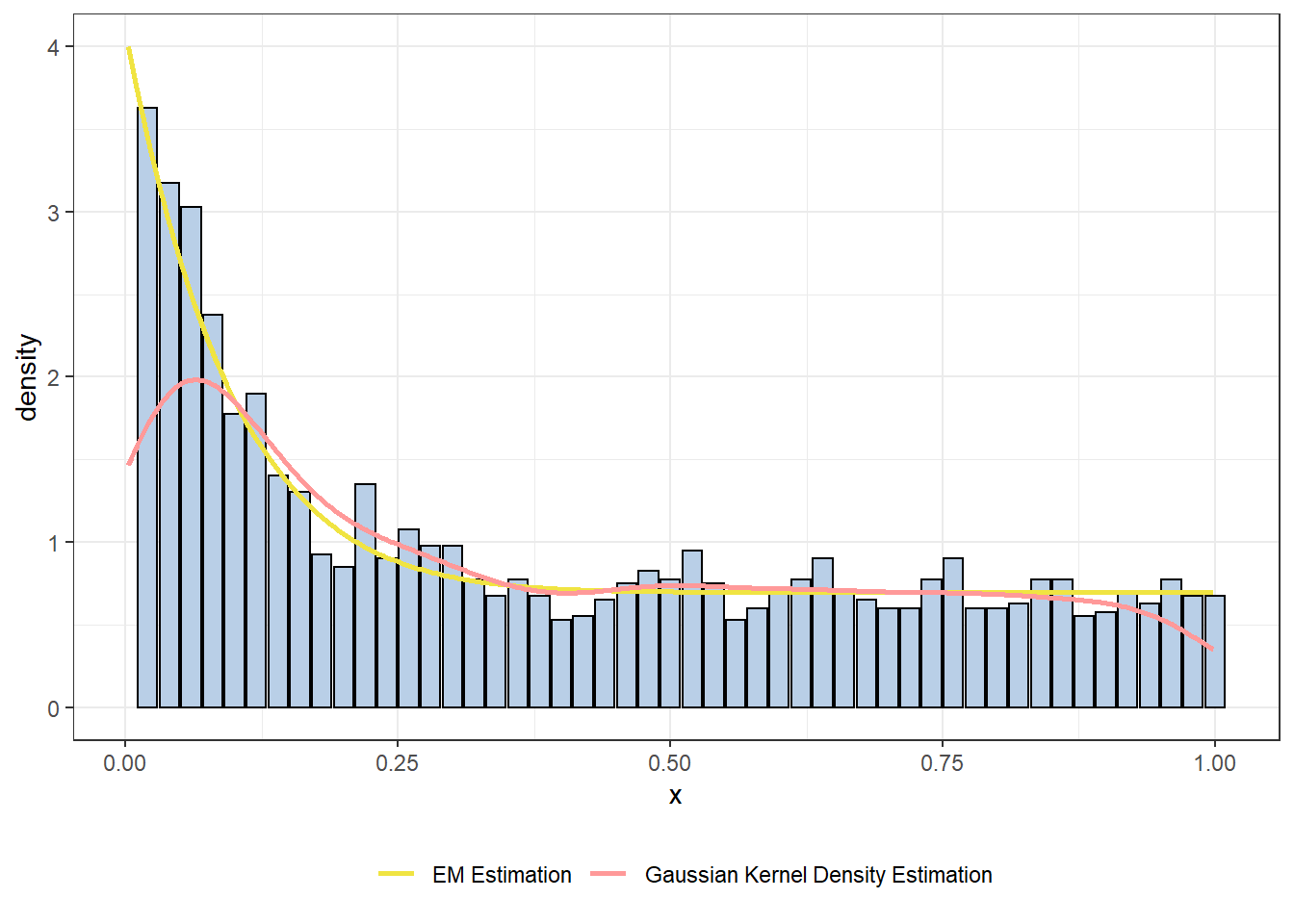
From the histogram, we can easily see that EM density estimation fits the real density very well. Not surprise to us, EM density estimation is a better choice comparing with Gaussian kernel density estimation for this data set.
2.3 Example - EM algorithm as a classification tool for mixture probabaility density.
We can classify \(x_i\) to be 1st group if \(T_{0,i}=P(z_i=0|\mathbf{x};\boldsymbol{\theta}^{(\text{32th iteration})}) \stackrel{(\text{A.}4)}{=} \frac{0.69679 \times 1}{0.69679 \times 1 + (1-0.69679) \times 11.09327(1-x_i)^{(11.09327 -1)}} > 0.5\).
Use R to calculate
pvalue["p0"] <- s.new[1]/(s.new[1] + (1-s.new[1]) * s.new[2] * (1-pvalue$X)^(s.new[2] - 1))
pvalue[pvalue$p0 >= 0.5, "estimated_group"] <- as.integer(0)
pvalue[pvalue$p0 < 0.5, "estimated_group"] <- as.integer(1)
pvalue[pvalue$group == pvalue$estimated_group,"Diff"] <- "Right classified"
pvalue[pvalue$group != pvalue$estimated_group,"Diff"] <- "False classified"
table(pvalue$Diff)
##
## False classified Right classified
## 321 1679The total number of false classified is \(321\). The false classified rate is \(321/(321+1679) = 0.1605\).
3 Appendix
For \(X\) and \(Y\) are random variables, \[\begin{equation} E[X+Y] = E[X] + E[Y] \tag{A.1} \end{equation}\]
For \(X\) is a random variable and \(a\) is a scalar, \[\begin{equation} E[aX] = aE[X] \tag{A.2} \end{equation}\]
For \(A\) is an event, \(\mathbf{I}_A\) is indicator function of the set \(A\),
\[\begin{equation} E[\mathbf{I}_A] = P(A) \tag{A.3} \end{equation}\]
For \(Z_i\) is group information, which is unknown and \(X_i\) is known data and both \(Z_i\) and \(X_i\) are considered as random variables.
\[\begin{equation} \begin{cases} T_{i,0} = P(Z_i = 0 | X_i = x_i; \tilde{\boldsymbol{\theta}}) = \frac{P(Z_i = 0 \cap X_i = x_i; \tilde{\boldsymbol{\theta}})} { P(X_i = x_i; \tilde{\boldsymbol{\theta}})} = \frac{\pi_0 f_0(x_i)}{\pi_0 f_0(x_i) + \pi_1 f_1(x_i)} \\ T_{i,1} = P(Z_i = 1 | X_i = x_i; \tilde{\boldsymbol{\theta}}) = \frac{P(Z_i = 1 \cap X_i = x_i; \tilde{\boldsymbol{\theta}})} { P(X_i = x_i; \tilde{\boldsymbol{\theta}})} = \frac{\pi_1 f_1(x_i)}{\pi_0 f_0(x_i) + \pi_1 f_1(x_i)} \end{cases} \tag{A.4} \end{equation}\]