Visualize ARIMA Model Selection
Kevin Liu
6/2/2018
#Library loading
library(ggplot2)
library(dplyr)
library(tidyr)
library(cowplot)
1 Beautiful ACF and PACF by ggplot2
Wolf yearly sunspot number is a classic time series data that have been analysis by many statisticians and scientists. In this blog, I want to emphasis on a graphic model selection method by Heiberger and Teles (2002) and Richard M. Heiberger (2015).
As shown in figure 1.1, the first to do in time series modeling is drawing plot for original data with its ACF and PACF plots. We notice that the orignal time series is stationary in mean but not stationary in variance. Box-cox data transformation is needed in Section 2.
data("sunspot.year")

arima.plot <- function(data = sunspot.year, title = "Main Title",lag.max = 24, ...) {
  if(class(data) != "ts") {stop("data must be ts")}

  df1 <- data.frame(value = as.numeric(data), time = as.numeric(time(data)))
  fig.main <- ggplot(data = df1, aes(x = time, y = value)) +
    geom_line() +
    ggtitle(title) +
    theme_bw() +
    theme(panel.grid.minor = element_blank(),
          plot.title = element_text(hjust = 0.5))

  list.acf <- acf(x = data, plot = FALSE, lag.max = lag.max)
  df.acf <- data.frame(lag = as.numeric(list.acf$lag), value = as.numeric(list.acf$acf))
  df.acf$type <- "ACF"

  list.pacf <- acf(x = data, type = "partial", plot = FALSE, lag.max = lag.max)
  df.pacf <- data.frame(lag = c(0,as.numeric(list.pacf$lag)), value = c(1,as.numeric(list.pacf$acf)))
  df.pacf$type <- "PACF"

  df.acf.pacf <- rbind.data.frame(df.acf, df.pacf)

  fig.merge <- ggplot(data = df.acf.pacf, aes( x = lag, y = value)) +
    geom_col(width = 0.2, fill = "#667fa2") +
    geom_hline(yintercept = qnorm((1+0.95)/2)/sqrt(dim(df.pacf)[1]),
               linetype = "dashed",
               colour = "grey50") +
    geom_hline(yintercept = -qnorm((1+0.95)/2)/sqrt(dim(df.pacf)[1]),
               linetype = "dashed",
               colour = "grey50") +
    scale_y_continuous(name = element_blank()) +
    scale_x_continuous(breaks = seq(0,24,4)) +
    facet_wrap(~type) +
    theme_bw() +
    theme(panel.grid.minor = element_blank(),
          strip.background = element_rect(fill = "#f8ddc4"))

  return(cowplot::plot_grid(fig.main, fig.merge, nrow = 2, rel_heights = c(2,1)))
}

arima.plot(title = "Sunspots from year 1700 to year 1988")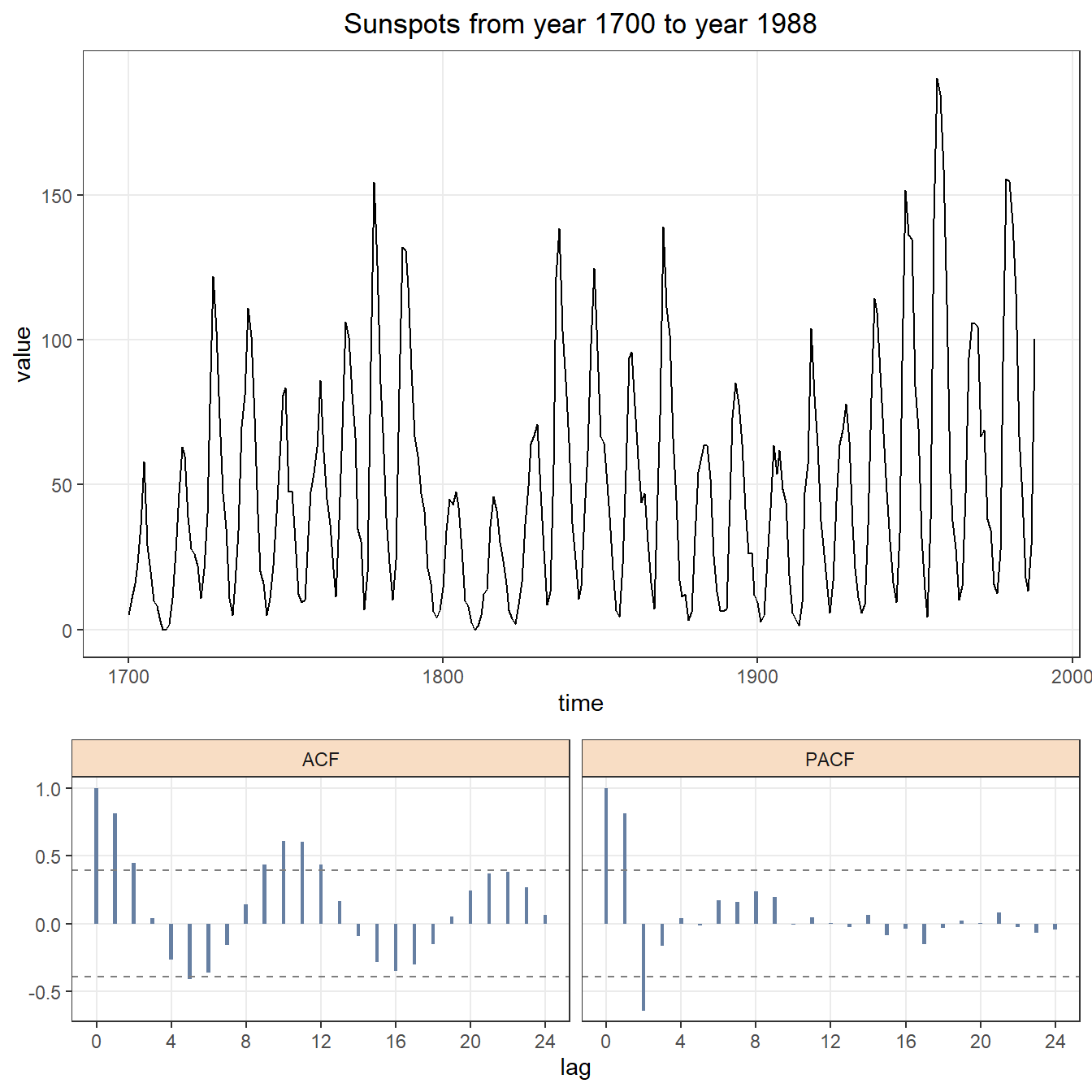
Figure 1.1: Time series plot with ACF and PACF
2 Data transformation
Using box-cox transformation method, we have that \(\hat{\lambda} = 0.46\). For the purpose of easy interpretation (people without statistic background will ask what does \(\hat{\lambda} = 0.46\) mean), we use \(\hat{\lambda} = 0.5\), which means that we should square root the original data,\(\sqrt{y_{t}}\). After transformation, variance becomes smaller, ACF tails off after lag 3 and PACF cuts off after lag 2, as shown in figure 2.2. This implies that ARIMA(3,0,2) should be a appropriate model for this data.
boxcox <- function(y, lambda = seq(-2, 2, 0.01), method = c("mle", "yule-walker", "burg", "ols", "yw"),...) {
  y = as.vector(y/(max(abs(y)) + 1))
  if (any(y <= 0))
    stop("y values must be positive")
  order <- ar(log(y), method = "mle")$order
  nlngmy <- sum(log(y))

  df.lambda <- data.frame(lambda = lambda)
  df.lambda.nonzero <- subset(df.lambda, lambda != 0 )
  list.var.pred <- lapply(X = t(df.lambda.nonzero$lambda), function(X) {
    ar((y^X - 1)/X,
       order.max = order,
       method = method)$var.pred
    })
  df.lambda.nonzero$var.pred <- unlist(list.var.pred)
  df.lambda.nonzero$loglik <- -length(y)/2 * log(df.lambda.nonzero$var.pred) +
    (df.lambda.nonzero$lambda - 1) * nlngmy
  df.lambda.zero <- subset(df.lambda, lambda == 0 )
  df.lambda.zero$var.pred <- ar(log(y), order.max = order, method = method)$var.pred
  df.lambda.zero$loglik <- -length(y)/2 * log(df.lambda.zero$var.pred) - nlngmy
  df.lambda <- rbind.data.frame(df.lambda.nonzero, df.lambda.zero)
  df.lambda <- df.lambda[order(df.lambda$lambda),]
  return(df.lambda)
}

df.lambda <- boxcox(y = sunspot.year + 1, lambda = seq(-3, 3, 0.01), method = "mle")
df.lambda.max <- df.lambda[df.lambda$loglik == max(df.lambda$loglik),]

ggplot(data = df.lambda, aes( x = lambda, y = loglik)) +
  geom_line() +
  geom_point( data = df.lambda.max) +
  geom_label( data = df.lambda.max, aes( x = lambda, y = loglik),
              nudge_y = -250,
              label = paste0(round(df.lambda.max$lambda,2),
                             " , ",
                             round(df.lambda.max$loglik,2))) +
  scale_x_continuous(breaks = -3:3) +
  theme_bw()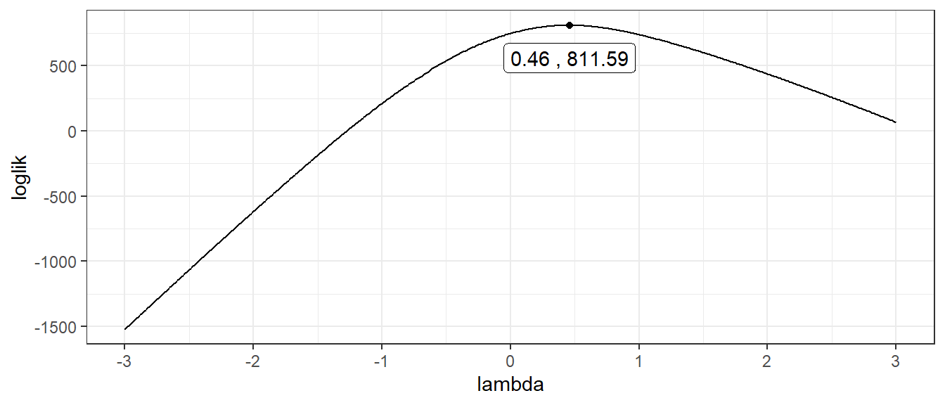
Figure 2.1: Box cox data transformation
sunspots.sqrt <- sqrt(sunspot.year)
arima.plot(data = sunspots.sqrt,title = "Sunspots from year 1700 to year 1988")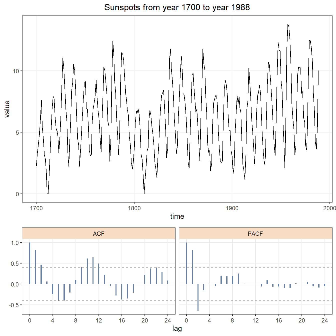
Figure 2.2: Square rooted time series with ACF and PACF
3 Visualized Model Comparison
The main purpose of this section is to determine which ARIMA is the most appropriate model based on residual analysis.
According to experience, for non-seasonal ARIMA mode, value of \(p\) and \(q\) won’t be larger than \(3\). I choose \(p = 3 \text{ and } q = 2\). After cartesian product of \(p \in (0,1,2,3)\) and \(q \in (0,1,2)\), we have \(4 \times 3 = 12\) possible ARIMA models, from ARIMA(0,0,0) to ARIMA(3,0,2).
From figue 3.1, we notice that ARIMA(0,0,0) - ARIMA(2,0,0) are not a good chioce since ACF and PACF are significant different from zero for many lags and residuals have large variance. Meanwhile, the difference from ARIMA(2,0,1) to ARIMA(3,0,2) is not very large, because those models have identical ACF, PACF and residual plots. More diagnosis are needed.
From figure 3.2, ARIMA(3,0,0) has the smallest AIC.
From figure 3.3, we have that results of goodness of fit test: Box-Pierce are very similar from ARIMA(2,0,1) to ARIMA(3,0,2).
Based all information and diagnosis we have, I feel confident to say that ARIMA(3,0,0) is the most appropriate model and that difference of ARIMA(2,0,1) - ARIMA(3,0,2) may not be large.
arima.order <- c(3,0,2)

p <- 0:arima.order[1]
d <- 0:arima.order[2]
q <- 0:arima.order[3]

df.arima.order <- data.frame(t(expand.grid(p=p,d=d,q=q)))
df.colnames <- data.frame(expand.grid(p=p,d=d,q=q))
df.colnames$type <- with(df.colnames,paste0("ARIMA(",p,",",d,",",q,")"))

list.arima.model <- lapply(df.arima.order,
                           function(data, x, ...) {
                             arima(x = data, order = x, ...)
                             },
                           data = sunspots.sqrt)

df.arima.residual <- sapply(list.arima.model,
                            function(x) {
                              x$residuals
                              })
df.arima.residual <- data.frame(df.arima.residual)
colnames(df.arima.residual) <- df.colnames$type
df.arima.residual$time <- time(sunspots.sqrt)

df.arima.residual.plot <- gather(data = df.arima.residual, value = "residual", key = "type",-time)

df.acf <- sapply(subset(df.arima.residual, select = -time),
       function(x, lag.max,...) {
         acf(x = x, lag.max = lag.max, plot = FALSE)$acf
       },
       lag.max = 24)
df.acf <- data.frame(df.acf)
colnames(df.acf) <- df.colnames$type

df.acf$lag <- 0:(dim(df.acf)[1]-1)
df.acf.plot <- gather(df.acf,
                      value = "value",
                      key = "Model",
                      -lag)


df.pacf <- sapply(subset(df.arima.residual, select = -time),
                  function(x, lag.max,...) {
                    acfvalue <- as.numeric(acf(x = x,
                                               lag.max = lag.max,
                                               type = "partial",
                                               plot = FALSE)$acf)
                    return(c(1,acfvalue))
                    },
                  lag.max = 24)
df.pacf <- data.frame(df.pacf)
colnames(df.pacf) <- df.colnames$type

df.pacf$lag <- 0:(dim(df.pacf)[1]-1)
df.pacf.plot <- gather(df.pacf,
                       value = "value",
                       key = "Model",
                       -lag)

fig.acf <- ggplot(data = df.acf.plot, aes(x = lag, y = value)) +
  geom_col(width = 0.4, fill = "#667fa2") +
  geom_hline(yintercept = qnorm((1+0.95)/2)/sqrt(dim(df.acf.plot)[1]),
             linetype = "dashed",
             colour = "grey50") +
  geom_hline(yintercept = -qnorm((1+0.95)/2)/sqrt(dim(df.acf.plot)[1]),
             linetype = "dashed",
             colour = "grey50") +
  scale_y_continuous(name = element_blank()) +
  scale_x_continuous(breaks = seq(0,24,4)) +
  ggtitle("ACF of residuals") +
  facet_wrap(~Model) +
  theme_bw() +
  theme(panel.grid.minor = element_blank(),
        strip.background = element_rect(fill = "#f8ddc4"))

fig.pacf <- ggplot(data = df.pacf.plot, aes(x = lag, y = value)) +
  geom_col(width = 0.4, fill = "#667fa2") +
  geom_hline(yintercept = qnorm((1+0.95)/2)/sqrt(dim(df.pacf.plot)[1]),
             linetype = "dashed",
             colour = "grey50") +
  geom_hline(yintercept = -qnorm((1+0.95)/2)/sqrt(dim(df.pacf.plot)[1]),
             linetype = "dashed",
             colour = "grey50") +
  scale_y_continuous(name = element_blank()) +
  scale_x_continuous(breaks = seq(0,24,4)) +
  ggtitle("PACF of residuals") +
  facet_wrap(~Model) +
  theme_bw() +
  theme(panel.grid.minor = element_blank(),
        strip.background = element_rect(fill = "#f8ddc4"))

fig.residual <- ggplot(data = df.arima.residual.plot, aes(x = time, y = residual)) +
  geom_line(colour = "#667fa2") +
  ggtitle("Residuals") +
  facet_wrap(~type) +
  theme_bw() +
  theme(panel.grid.minor = element_blank(),
        strip.background = element_rect(fill = "#f8ddc4"))

cowplot::plot_grid(fig.acf, fig.pacf, fig.residual, nrow = 3)
## Don't know how to automatically pick scale for object of type ts. Defaulting to continuous.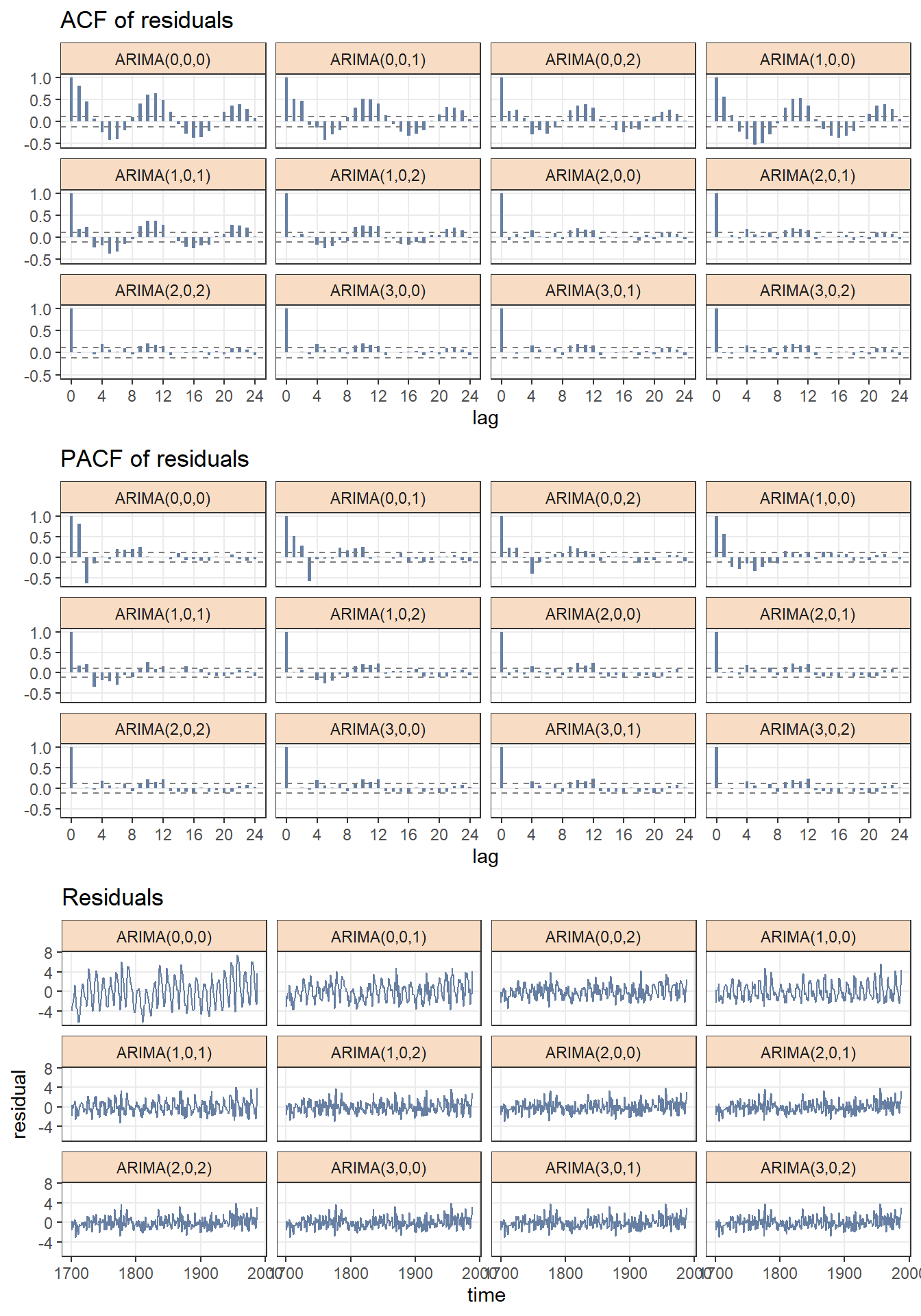
Figure 3.1: Residual diagnostics
aic <- sapply(list.arima.model, function(X) {X$aic})
aic <- round(as.numeric(aic),2)
df.aic.plot <- data.frame(aic = aic, p = df.colnames$p, q = df.colnames$q)

ggplot(data = df.aic.plot, aes(x = p, y = q)) +
  geom_raster(aes(fill = aic)) +
  geom_text(aes( label = aic), colour = "white") +
  scale_x_continuous(expand = c(0.05,0.05)) +
  scale_color_continuous( high = "#FFA800", low = "#4AC200") +
  theme_bw() +
  theme(panel.grid.minor = element_blank()) +
  scale_fill_distiller(palette = "Spectral", direction = -1)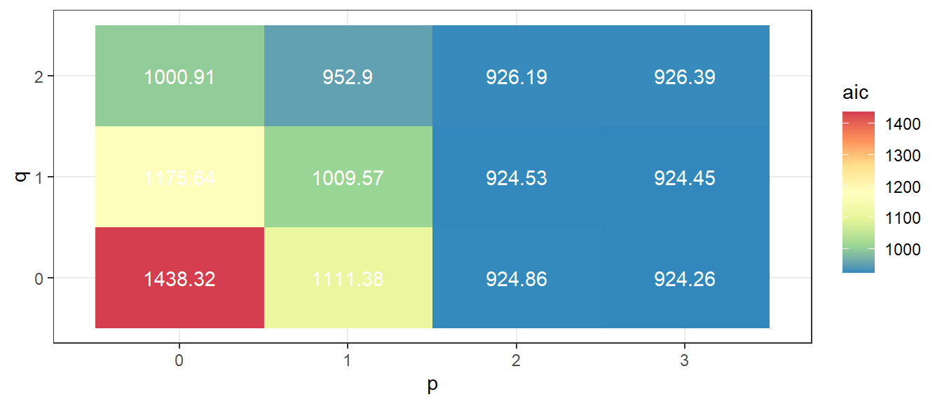
Figure 3.2: Information criteria
df.box.test <- sapply(list.arima.model, function(x) {
  residuals <- x$residuals
  df.lag <- data.frame(t(1:24))
  as.numeric(sapply(df.lag, function(maxlag) {
  pvalues <- Box.test(x = residuals, lag = maxlag)$p.value
  return(pvalues)
}))
})

df.box.test <- as.data.frame(df.box.test)
colnames(df.box.test) <- df.colnames$type
df.box.test$lag <- 1:24

df.box.test <- gather(df.box.test, value = "p.value", key = "model.type", -lag)

ggplot(data = df.box.test, aes(x = lag, y = p.value)) +
  geom_point(colour = "#667fa2") +
  facet_wrap(~model.type) +
  scale_x_continuous(limits = c(0,24), breaks = seq(0,24,6)) +
  theme_bw() +
  theme(panel.grid.minor = element_blank(),
        strip.background = element_rect(fill = "#f8ddc4"))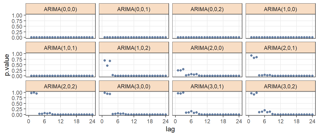
Figure 3.3: Goodness of fit:Box-Pierce
References
Richard M. Heiberger (2015) Heiberger and Teles (2002) Wei (1990)